
series: AI from zero to expert | article 7 of 30Training is not feeding data to a machine and hoping. It is a process with rules.
What training actually means
Chapter 6 left four algorithms on the table and one phrase repeated without ever being unpacked, “it gets trained on the data”. Time to open that box. Training a model is the process by which an algorithm adjusts its own internal numbers, its parameters, until its predictions on a set of examples match the known correct answers as closely as possible.
Put that way it sounds like magic. It is not, it is a fairly dumb loop repeated an enormous number of times. The model makes a prediction, it gets compared against the real answer, the size of the mistake is measured by something called a loss function, and the parameters get nudged in whichever direction reduces that mistake. Again. And again. The process ends when the error stops dropping meaningfully, or when the time and compute budget runs out, which in practice is the deciding factor more often than anyone likes to admit.
The loop is not the important part of this chapter. Everything around it is, the decisions made before and after, because that is where a machine learning project is won or lost. What data goes in, in what shape it goes in, how you check the result is worth anything, and why a model that gets everything right is usually a sign that something has gone very wrong.
Walking downhill in fog
The standard analogy for parameter fitting is a mountain, and it works because the problem is literally geometric. Picture a landscape of hills and valleys where the height at any point represents how wrong the model is with one particular combination of parameters. Valleys are good configurations, low error. Peaks are bad ones. Training means finding the bottom of a valley.
The catch is that you cannot see the landscape. You are standing somewhere in thick fog, and all you can do is feel the ground under your feet to work out which way is downhill, take a step that way, and repeat. That is gradient descent, the procedure that powers modern machine learning. The “gradient” is the direction of steepest slope at that exact spot, and the algorithm computes it, moves a little the opposite way, and looks again.
The size of each step matters enormously and it is called the learning rate. Steps too small and training takes forever to reach the bottom. Steps too large and the model bounces from one side of the valley to the other without ever settling, or shoots straight back up the slope. There is no universally good value, it depends on the problem.
The other complication of the fog is that you can end up at the bottom of a small dip convinced it is the lowest point in the whole landscape. In jargon, a local minimum instead of the global one. For years that was assumed to be the great obstacle in training, and a paper by Yann Dauphin and colleagues presented at NeurIPS 2014 argued otherwise. In very high-dimensional spaces, critical points are overwhelmingly more likely to be saddle points than genuine local minima. A saddle point goes down in some directions and up in others, and surrounded by nearly flat plateaus it can stall training for a long stretch while giving the false impression of having reached the bottom. The risk of getting stuck is still real, and it explains why two training runs of the same model from different starting points can land in different places.
Parameters and hyperparameters are not the same thing
Two words that sound alike and get mixed up constantly are worth separating.
Parameters are the numbers the model learns by itself during training. The coefficients of a regression, the weights of a neural network. Nobody writes them by hand, they come out of the loop above. When someone says a language model has seventy billion parameters, this is exactly what they mean, the count of adjustable numbers inside it.
Hyperparameters are the configuration decisions made before training that the model cannot learn on its own. The learning rate from the previous section is a hyperparameter. The maximum depth of a decision tree, a hyperparameter. How many groups k you ask k-means for, a hyperparameter. They are the knobs on the control panel, and setting them well has as much impact on the final result as picking the algorithm.
The crude way to tune them is to try combinations by brute force and keep the best one. There are more elegant methods, but they all share one requirement that leads straight into the next section, comparing configurations needs data the model has not seen, and it must not burn the data you set aside for the final evaluation.
Data goes in as features
An algorithm does not understand “a house”, or “a customer”, or “an email”. It understands numbers. Translating a real-world object into a list of numbers the algorithm can digest is what gets called a feature representation. Each feature is a column, one measurable variable of the object.
For a house the obvious features are floor area, number of rooms, year built, storey. For an email they might be the number of links, the presence of certain words, the time it was sent, whether the sender is in the address book. That list of numbers per example is exactly the vector chapter 4 talked about, and the model never sees anything else.
This is where the part of the craft that no tool fully automates shows up, feature engineering. It means deciding what gets measured and how it gets transformed before handing it over. A concrete example, if you have a customer’s date of birth, feeding the model the number 19870324 tells it nothing useful. Converting it to an age does. And on some problems, converting it into age brackets says more than the exact age. The information is the same, the shape it arrives in completely changes what the model can learn from it.
Some transformations are not optional. If one feature runs from 0 to 1 and another from 0 to 500,000, many algorithms will treat the second as vastly more important purely because of the scale of its numbers, with no underlying reason. So they get normalised, brought onto a comparable range. Non-numeric variables like country or product type need their own conversion, one that does not invent a false ordering, because coding Spain as 1 and France as 2 quietly tells the model that France is twice as much of something.
This unglamorous, highly manual prep work eats an enormous share of the time on a real project. A note of precision is owed on the figure repeated in talks and articles, the one about data scientists spending 80% of their time cleaning data. That number circulates without a clear primary source behind it. Industry surveys that do publish time breakdowns, such as Anaconda’s State of Data Science, have put data preparation somewhere around 40 to 45% of the working day depending on the year. It is still the single most expensive activity, and it is still not the 80% everyone quotes from memory. Chapter 9 digs into why this phase weighs so much.
The dataset gets split in two, at minimum
Here is the idea that separates someone who has trained a model from someone who has trained a model that is worth anything.
If you train on all the data you have and then measure accuracy on that same data, the number you get means nothing. It is like marking an exam taken by someone who studied the answers to that specific exam. A good score does not prove they understood the subject, it proves they have a good memory.
The standard fix is to split the data before you start. One part, the bulk of it, is used for training. Another, which the model never sees during training, is held back to evaluate it afterwards. That held-out part is the test set, and its score is the only one worth taking seriously, because those examples are new to the model. Serious projects add a third split, the validation set, used for intermediate decisions like choosing between configurations, so that the test set is touched exactly once at the end and stays a clean exam.
When data is scarce, holding a chunk back hurts. That is what cross-validation is for, formalised by M. Stone in 1974 in the Journal of the Royal Statistical Society. The idea is to split the data into several blocks, train several times rotating which block plays the exam, and average the results. Every example ends up used for both training and evaluation, just never at the same time in the same round.
There is a silent way to break all of this and it has a name, data leakage. It happens when information from the test set seeps into training without anyone noticing, for instance if you normalise all features using the mean of the whole dataset before splitting it, or if the same customer appears on both sides under different records. The symptom is a suspiciously good test result followed by a faceplant in production.
A particularly treacherous variant shows up with time-ordered data. If you are predicting which customers will churn next month and you scatter the rows randomly across training and test, the model ends up training on March to predict February. It looks brilliant on the exam. In reality, where the future has not happened yet, it does not have that advantage. With time series the split goes by date, train on the past, evaluate on the future, exactly how it will work the day it ships.
And one detail gets forgotten the moment you leave the lab. The world changes, so a model trained on data from two years ago can degrade without anyone touching a line of code, simply because the behaviour patterns it learned are no longer current. That phenomenon is called drift, and it is why a model in production is not a finished product but something you have to watch and retrain.
Overfitting, when the model memorises
A model can fail in two opposite ways, and both have names.
Underfitting is the easy one to spot. The model is too simple for the pattern in the data, and it fails everywhere, training included. Trying to describe with a straight line something that clearly draws a curve. It gets caught quickly because the numbers are bad from the start.
Overfitting is the real problem. The model has enough capacity to learn the training data by heart, example by example, noise, measurement errors and coincidences included. On training it gets almost everything right. On new data it collapses. It learned the exam, not the subject.
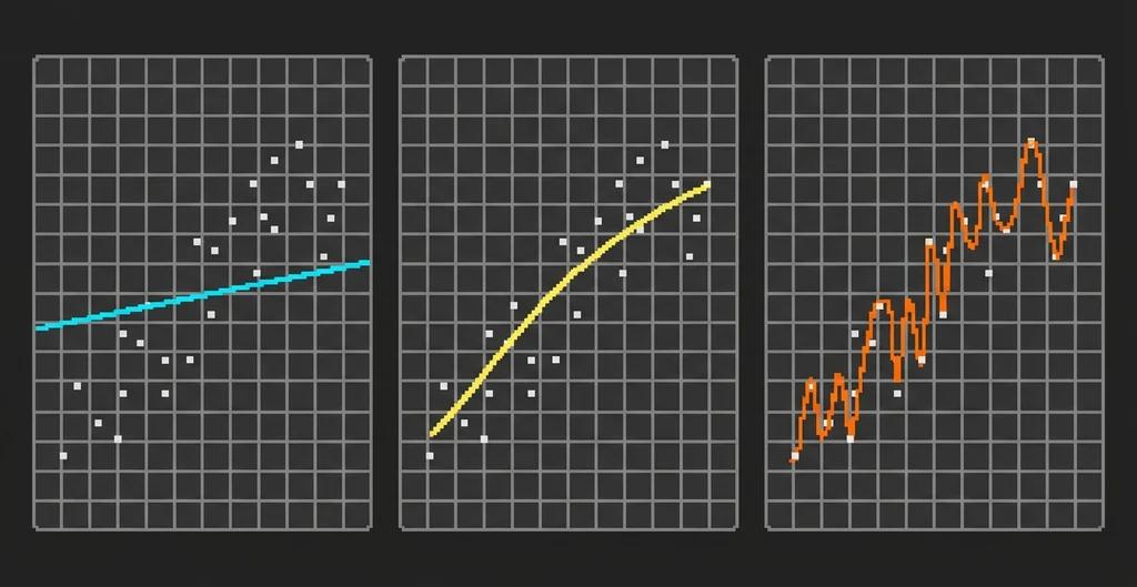
Between those two extremes sits a tension with a formal treatment in the field. Stuart Geman, Elie Bienenstock and René Doursat described it in 1992 in “Neural Networks and the Bias/Variance Dilemma”, published in Neural Computation, as the trade-off between bias and variance. A very rigid model has high bias, it always gets things wrong the same way because its shape cannot do better. A very flexible model has high variance, it changes drastically if you nudge the training data, because it is adapting to details that do not matter. The sweet spot is in between, and finding it is a good chunk of the job.
The tools against overfitting are several and all point the same way, restrict the model’s freedom or give it more examples. More training data, because the more varied what it has seen, the less it can memorise. Regularisation, mathematical penalties on needlessly complicated models. Early stopping, cutting training off when validation error starts rising while training error keeps falling, which is the classic signal that memorisation has begun. And for the trees of the previous chapter, pruning and forests.
There is no best algorithm
One reasonable question remains. Given four classic algorithms and many more that did not fit in chapter 6, which is the good one?
The answer has a mathematical proof and it tends to disappoint. David Wolpert published work in Neural Computation in 1996 that is popularly known as the “no free lunch” theorem for learning. Its conclusion, put briefly and losing some precision on the way, is that no learning algorithm is superior to another when averaged over all possible problems. For every problem where A beats B, another exists where B beats A.
What that means in practice is not that your choice is irrelevant. It means an algorithm’s superiority is always relative to a type of problem and a particular shape of data, never absolute. Which is why the real workflow is not picking the best algorithm on paper, it is trying several reasonable candidates on the same data, split the same way, and comparing their results with the same metric.
And that is where the next trap appears, the one that fills chapter 8 entirely. Comparing results means choosing a metric, and the wrong metric can make a useless model look excellent.