
series: AI from zero to expert | article 6 of 30Four algorithms that have been working for decades without a single neural network.
The toolbox
Chapter 5 laid out the three schools of machine learning, supervised, unsupervised and reinforcement. Those were three ways of framing a problem, not three ways of solving one. This chapter goes down a floor into the engine room, the classic machine learning algorithms that have been solving real problems inside those schools for decades.
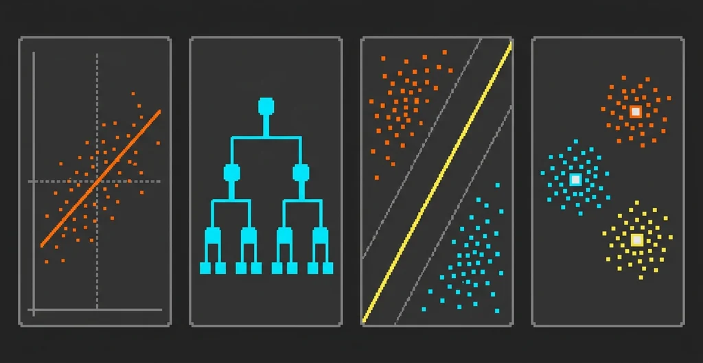
Four names that show up in every machine learning syllabus and every data science job ad, regression, decision trees, support vector machines and k-means. The first three are supervised, the fourth is unsupervised. None of the four is a neural network and none of the four needs a GPU to run.
One widespread misconception is worth killing off right at the start. These algorithms are not the prehistory of AI, and they are not a mandatory stop on the way to the good stuff. They run today, in production, inside companies that also have deep learning models humming away in the same building. The reason is at the end of this chapter, backed by a recent benchmark. First, what each one actually does.
Regression, the line that fits best
Regression is the oldest of the four by a comfortable margin of nearly two centuries. The least squares method, its mathematical engine, was first published in 1805, in an appendix titled “Sur la Méthode des moindres quarrés” inside a book by Adrien-Marie Legendre about calculating the orbits of comets. No computers, no massive datasets, just astronomers trying to fit a curve through a handful of observations taken by hand through a telescope.
The word “regression” arrived eighty years later, by an unexpected route. Francis Galton published a study on inherited height in the Journal of the Anthropological Institute in 1886, where he noticed that children of very tall parents tended to be tall, but less tall than their parents, and children of very short parents tended to be short, but less short than theirs. Heights “regressed” towards the population average. That biological observation is where the entire machine learning industry got the word it now uses for something considerably less romantic than heredity.
The idea is easy to picture. You have a cloud of points on a chart, say house size on one axis and price on the other. Linear regression looks for the line that passes as close as possible to all those points at once. “As close as possible” has a precise definition, you measure the vertical distance from each point to the line, square it so that errors above and below do not cancel each other out, and hunt for the line that minimises the sum of all those squares. Hence the name of the method.
Once the line is drawn, prediction is trivial. A new house arrives with a given size, you read off the matching price on the line, and there is your estimate. In practice there is rarely a single input variable, more like dozens (size, number of rooms, age, distance to the centre), and the line stops being a line and becomes a plane or its equivalent in higher dimensions. The intuition does not change, you are still hunting for the surface that best fits the cloud.
There is a variant for classification, logistic regression, which despite the name solves a different problem. Instead of spitting out any number at all, it squeezes its output into a value between 0 and 1 that reads as the probability of belonging to a class. It is the algorithm that answers “how likely is it that this email is spam” with a number rather than a flat yes or no, and it is still the first tool anyone reaches for on a huge share of binary classification problems in industry.
The big advantage of regression is interpretability. A trained model is literally a list of coefficients, one per variable, and each coefficient tells you how much the prediction moves when that variable changes. You can walk a business stakeholder through the model and have them understand why it predicts what it predicts. That conversation is considerably more awkward with a billion-parameter neural network.
The big limitation is the flip side of the same coin. Linear regression assumes the relationship between inputs and output is a straight line, and the real world is full of relationships that are anything but. When the data has a twisted shape, the best possible line is still a bad line.
Decision trees, a questionnaire that writes itself
A decision tree works like a chained questionnaire. Is the transaction over 500 euros? If yes, was it made outside the customer’s usual country? If yes, did it happen between 3 and 5 in the morning? Every answer routes you to another question, until you reach the end of a branch, where a conclusion sits. Fraud, or not fraud.
The structure is not the interesting part, anyone could sketch that on a napkin. The interesting part is that the algorithm decides on its own which questions to ask and in what order, straight from the training data. At each node it tries every possible split of every available variable and keeps the one that separates the data best, the one leaving the resulting groups “purest”, with the least class mixing. Then it repeats inside each group, and keeps going until further splitting stops paying off.
How that purity gets measured is exactly where the history of the algorithm forks, because decision trees were developed twice in parallel, in two communities that barely read each other. On the statistics side, Leo Breiman, Jerome Friedman, Richard Olshen and Charles Stone published the book “Classification and Regression Trees” in 1984, which gave the CART approach its name and which measures purity with the Gini index. On the machine learning side, Ross Quinlan published “Induction of Decision Trees” in 1986, in the very first volume of the journal Machine Learning, describing the ID3 system, which measures purity with entropy borrowed from information theory. Two cultures, two vocabularies, the same animal.
Trees have one virtue no other algorithm on this list matches. They are genuinely auditable. You can print the trained tree, read it top to bottom and explain every single decision the model makes with a finger on the paper. In sectors where an automated decision has to be justified to a regulator or to a customer, that is not a cosmetic detail, it is a requirement.
They also have a serious flaw. A tree left to grow unchecked ends up inventing a bespoke question for every single training example, memorising instead of learning. That is the problem chapter 7 will name properly, overfitting. The usual fix is not pruning one tree into perfection, it is the elegant brute force of training hundreds of different trees, each on a different slice of the data and the variables, and having them vote. That is a random forest, and its more aggressive cousin, gradient boosting, builds the trees in a chain, each one specialised in cleaning up the errors the previous one left behind. Modern implementations of this family are the ones that keep turning up at the top of tabular data competitions. The best known is XGBoost, presented by Tianqi Chen and Carlos Guestrin in 2016, which its own authors describe as a system widely used by data scientists to reach state-of-the-art results on machine learning challenges.
SVM, the widest possible corridor
Support vector machines, SVM for short, solve a classification problem with a very concrete geometric idea. If you have two groups of points and you want to separate them with a line, there are infinitely many lines that do the job. The question an SVM asks is which of all those lines is the best one, and its answer is the one leaving the widest corridor between the two groups. In jargon, the one that maximises the margin.
The intuition behind that choice is solid. A boundary drawn tight against the points of one group will work on the training data, but any new example nudged slightly out of place lands on the wrong side. A boundary sitting in the middle of a wide corridor has room for error on both sides. The points touching the edge of that corridor, the ones right at the limit of what is possible, are the “support vectors” the algorithm is named after. Every other point, comfortably deep inside its own group, has zero influence on where the line ends up. The algorithm is defined by its edge cases.
The training algorithm was presented in 1992, in “A Training Algorithm for Optimal Margin Classifiers” by Bernhard Boser, Isabelle Guyon and Vladimir Vapnik, at the COLT workshop. That same paper carries the piece that turned SVMs into the reference algorithm of an entire era, the kernel trick. Three years later, Corinna Cortes and Vladimir Vapnik published “Support-Vector Networks” in the journal Machine Learning, adding the soft margin, the tolerance for some points falling on the wrong side of the boundary. That is what made the method usable on data that cannot be cleanly separated, which is the normal situation outside a textbook example.
The kernel trick deserves its own explanation. Picture red and blue points on a table, with the red ones forming a ring around the blue ones. There is no straight line on that table that separates them. But if you lift the blue points up above the table and leave the red ones down, suddenly a flat sheet of paper does the job. The kernel trick does exactly that, it projects the data into a space with many more dimensions where a flat boundary does exist, and it does so without ever computing those new coordinates explicitly, which would be ruinously expensive. It works only with the distances between pairs of points, which is all it actually needs.
The cost of SVMs shows up with volume. Training scales badly once the number of examples climbs into the millions, and that is where other families of algorithms take the ground back.
K-means, grouping without knowing what you are looking for
The only unsupervised one of the four. Chapter 5 already introduced the name and the job it does, grouping unlabelled data into clusters of items that resemble each other. Here comes the mechanism, which is surprisingly short to describe.
You choose how many groups you want, and that number is k. The algorithm drops k centres at starting positions, and from there it loops over two steps. First, it assigns every point to whichever centre is nearest, forming k groups. Second, it moves each centre to the midpoint of all the points that landed with it. That movement changes the distances, so some points now sit closer to a different centre, and the loop starts again. It repeats until the centres stop moving. At that point the algorithm has converged and the groups are formed.
The origin of the procedure is a curious case of delayed publication. Stuart Lloyd described it in 1957 in an internal Bell Labs technical report, applied to a telecommunications problem with nothing to do with grouping customers, the quantisation of signals in pulse-code modulation. That report did not appear as a formal publication until 1982, in IEEE Transactions on Information Theory, twenty-five years later. The name “k-means” was coined by James MacQueen in 1967, in the same Berkeley Symposium paper cited in the previous chapter.
The two weaknesses of k-means fall straight out of its own mechanism. First, you pick k, the algorithm does not discover it. Ask for three groups from data that naturally has five and you will get three groups anyway, no complaints. Second, the result depends on where the initial centres land, so in practice you run it several times from different starting points and compare.
Why they are still here
That leaves the awkward question. If neural networks can generate video and write code, why would anyone in 2026 train a tree model to predict default rates across a loan book?
The answer has recent empirical backing. Léo Grinsztajn, Edouard Oyallon and Gaël Varoquaux published an extensive benchmark at NeurIPS 2022 comparing tree-based models against deep learning methods on tabular data, those tables of rows and columns that are the daily bread of banks, insurers, hospitals and retailers. Their conclusion was that tree-based models remain state of the art on medium-sized datasets, around ten thousand examples, and that the gap is not explained away by categorical features and does not disappear once you tune the networks properly.
Then there are the less scientific and very real reasons. A logistic regression trains in seconds, fits on any server, needs no GPU rented by the hour, and when it fails you can work out why. A tree model can be audited in front of a regulator. A k-means over purchase history answers a concrete business question in an afternoon. Picking an enormous model for a small problem is not sophistication, it is spending.
Chapter 7 picks up the thread this one kept dropping. Whichever classic machine learning algorithms you pull out of this toolbox, they all share the same training process and they can all fall into the same trap, memorising the examples they have already seen instead of learning the pattern underneath.
Sources
– J. Ross Quinlan, “Induction of Decision Trees”, Machine Learning 1 (1986), pp. 81-106
– Corinna Cortes y Vladimir Vapnik, “Support-Vector Networks”, Machine Learning 20 (1995), pp. 273-297
– Tianqi Chen y Carlos Guestrin, “XGBoost: A Scalable Tree Boosting System”, KDD (2016)