series: AI from zero to expert | article 4 of 30Before we get into classic machine learning, neural networks, and language models, this chapter takes a different shape: no history, no philosophy, just the minimum toolkit of math for AI you need for the rest of the series to actually click. No heavy formulas, no exams, no flashbacks to university. Just the intuition behind three ideas: vectors, matrices, and probability.
It’s not a coincidence that modern AI leans on exactly these three branches of math and not others. Linear algebra (vectors and matrices) gives a compact, highly efficient way to represent and transform huge amounts of data at once, something computers happen to be especially fast at thanks to hardware built for exactly that. Probability, for its part, gives a formal language for a system to express how sure or unsure it is about something, instead of faking a certainty it doesn’t have. Between the two, they cover, at the intuition level, almost everything you need for the rest of this series to make sense.
Vectors
A vector, in its simplest form, is an ordered list of numbers. Nothing more exotic than that. Geometry adds a useful extra layer of intuition: a vector can also be thought of as an arrow with a specific direction and magnitude, anchored in a space with as many dimensions as the list has numbers. That double reading (list of numbers on one hand, arrow in space on the other) is the backbone of Grant Sanderson’s “Essence of Linear Algebra” video series, better known as 3Blue1Brown, which remains, years after it was published, one of the most cited explanations of this idea online.
Why does any of this matter to AI? Because almost everything a model processes gets turned into vectors first. An image becomes a very long vector of pixel intensity values. A word becomes a vector of numbers that captures, in some abstract way, its meaning. That second case has an example that’s become famous in the field: in 2013, a Google team made up of Tomas Mikolov, Kai Chen, Greg Corrado, and Jeffrey Dean published a system called word2vec, capable of representing words as vectors in a way that relationships between meanings behaved like arithmetic operations. The example that shows up in every introduction to the topic, documented in a related paper by Mikolov together with Wen-tau Yih and Geoffrey Zweig: take the vector for “king,” subtract the vector for “man,” add the vector for “woman,” and the result lands very close to the vector for “queen,” without anyone ever explaining to the system what royalty or gender are. Worth the honest caveat: that clean result depends on excluding the original words from the nearest-neighbor search. If you don’t exclude them, the closest result is usually, literally, “king” again. Caveat aside, the underlying idea holds up and remains one of the most cited demonstrations that meaning can be captured, to some extent, with numbers and geometry.

Once any two things (two words, two images, two users of an online store) are represented as vectors, a very practical question shows up: how similar are they? The usual answer is to measure the angle between both vectors, not the distance between their tips. The smaller the angle, the more they point in the same direction, the more “alike” they are in whatever that space represents. This is called cosine similarity, and it’s literally the mechanism behind a basic recommendation engine: your tastes get turned into a vector, so do thousands of products, and the system recommends whatever points in a direction closest to yours. You don’t need to remember the technical name. What’s worth keeping is the idea: in vector space, “similar” has a concrete geometric definition, not a vague feeling.
The vectors real AI models work with almost never have two or three numbers, like the examples drawn on a whiteboard with arrows. A modern language model typically represents each word with a vector of several hundred, or even thousands, of numbers. Nobody can draw or mentally picture an arrow in a 1,536-dimensional space, and you don’t need to: the math of vectors, angles, and distances works exactly the same with two dimensions as with fifteen hundred, even though our geometric intuition runs out past the third. The whiteboard arrow is just scaffolding for the idea, not an actual limit on the concept.
Matrices
If a vector is a list of numbers, a matrix is a table of numbers, rows by columns. But the most useful way to think about a matrix, for where this series is going, isn’t as a static table of data, it’s as a function: something that takes a vector and turns it into a different one. Multiplying a vector by a matrix moves it to a new spot in space, stretches it, rotates it, or squashes it, depending on what numbers the matrix holds. A very simple matrix can, for instance, take any vector and flip it backward, double all its values, or squash it down to almost a single point. Each of those geometric operations corresponds to a specific table of numbers.
When a photo app rotates an image, straightens it, or stretches it to fit a different frame, underneath it’s applying exactly this kind of transformation to the table of numbers that represents that image, pixel by pixel. The difference between that and a neural network isn’t the type of operation (multiplying vectors by matrices), it’s that in a neural network nobody hand-picked the matrix’s numbers to get a specific effect like “rotate 90 degrees”: those numbers adjust themselves, automatically, during training, until the resulting transformation does what it was asked to do (recognize a cat, translate a sentence, whatever), without any human writing that rule explicitly. It’s the same math you use without knowing it every time you rotate a photo on your phone, just applied at a completely different scale and for a completely different purpose.
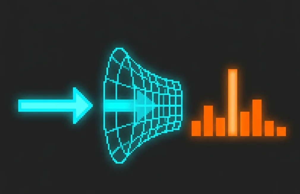
This idea is literally what a neural network does, layer by layer (you’ll see it in detail in chapter 11): each layer applies a matrix transformation to the data it receives, and training the model is nothing more than adjusting the numbers inside those matrices (the model’s “weights”) until the full transformation, start to finish, turns an input (an image, a piece of text) into the right output. When you read that a language model has “70 billion parameters,” what’s actually being described is the total size of all those matrices added up: 70 billion individual numbers, each one tuned during training so the full transformation works. The most cited academic reference on this, Mathematics for Machine Learning, by Deisenroth, Faisal, and Ong (Cambridge University Press, 2020, free online), spends its opening chapters building exactly this intuition before touching a single machine learning algorithm. That order isn’t an accident: skip it, and everything that follows gets memorized instead of understood.
Vectors and matrices also share a more general name you’ll run into constantly the moment you read or look at AI code: tensor. A tensor is nothing more than a generalization of the same idea to any number of dimensions: a single number is a tensor of order zero, a vector is a tensor of order one, a matrix is a tensor of order two, and a table of numbers with three, four, or more axes (say, a collection of color images, which needs one axis for height, one for width, one for color, and one more for how many images there are) is a higher-order tensor. You don’t need to picture it geometrically beyond the matrix, it’s enough to hold onto the idea of a table of numbers with several axes. The name isn’t a coincidence: the two most-used programming libraries for building AI models are called TensorFlow (Google’s) and PyTorch, whose core data type is called, literally, a tensor. Everything you’ve seen in this section about vectors and matrices is, at bottom, the simplest special case of that same idea.
Probability
Probability is the third piece, and it’s the odd one out because it doesn’t describe objects (vectors, matrices), it describes uncertainty. A machine learning model almost never gives you an answer with one hundred percent certainty: it gives you a probability, a number between 0 (impossible) and 1 (certain), that something is true. The spam filter from chapter 1 doesn’t decide, in a flat binary way, that an email is spam: it calculates a probability that it is, and applies a threshold (say, above 90%, it goes to the spam folder) to turn that probability into a concrete decision. That threshold is a design choice, not a law of physics, and moving it up or down changes how many legitimate emails get flagged as spam and how much real spam slips through as legitimate: raising the threshold cuts false positives but lets more real spam through, lowering it does the opposite. There’s no universal “correct” threshold, only different trade-offs depending on which kind of error worries you more. We’ll come back to this threshold, by name and in detail, in the evaluation metrics of chapter 8.
A model’s probability isn’t a measure of objective truth about the world, it’s a measure of the model’s own confidence, calculated from the data it was trained on. A model can be very confident (a high probability) and still be wrong, if its training data had gaps or bias. High probability isn’t a synonym for guaranteed truth, it’s a synonym for “this closely matches the patterns this particular model has seen before.”
You don’t need any AI data to see why this distinction matters, just arithmetic. Picture a medical test with 99% accuracy for detecting a disease that affects 1 in every 10,000 people. If you test positive, what’s the probability you actually have it? Intuition says almost 99%. The arithmetic says something else: out of 10,000 people, only 1 actually has the disease (and the test likely catches it), but out of the 9,999 healthy people, 1% (about 100 people) will still get a false positive. So out of roughly 101 total positives, only 1 is real: the probability of actually being sick after a positive result lands around 1%, not 99%. This has a name in statistics, the base rate fallacy: ignoring how rare a starting condition is leads to wildly overestimating how reliable a positive result is. That same kind of arithmetic, applied at the scale of millions of automated decisions (a bank’s fraud detection system, a content filter, an image-based diagnosis), is exactly what makes a model’s accuracy, on its own, without context on how frequent whatever it’s detecting actually is, a number that misleads very easily. We’ll come back to this in more detail, with concrete names for each type of error, in chapter 8.
We’re leaving out differential calculus (derivatives, gradients) to cover in later chapters. We’re also not getting into statistics beyond basic probability here.
And this is where the three pieces stop being three separate chapters and become a single pipeline, which is roughly how a modern language model actually works: your text turns into vectors, those vectors pass through layer after layer of matrices that keep transforming them, and at the end of that pipeline the model doesn’t spit out one fixed word, it spits out a different probability for every possible word in the language, and picks (or nearly picks, with some calculated randomness thrown in) the most likely one, or one of the most likely ones. Vector, matrix, probability, in that order, over and over, layer after layer.
With these three pieces (vectors as a way to represent information, matrices as a way to transform it, probability as a way to quantify how uncertain the result is), you have the minimum math for AI you need for the rest of this series to stop sounding like magic and start sounding like engineering, which is what it actually is. You don’t need to be able to multiply two matrices by hand or memorize Bayes’ theorem to follow the rest of this series. You just need these three words (vector, matrix, probability) to stop sounding like jargon and start sounding like tools with a specific job to do, because you’re going to see them show up again and again in the coming chapters, applied to increasingly concrete problems.
Next chapter really kicks off phase 1: supervised, unsupervised, and reinforcement learning, the three schools of classic machine learning.
Sources
- Grant Sanderson (3Blue1Brown), “Essence of Linear Algebra”
- Mikolov, Chen, Corrado, Dean, “Efficient Estimation of Word Representations in Vector Space” (2013)
- Mikolov, Yih, Zweig, “Linguistic Regularities in Continuous Space Word Representations” (NAACL 2013)
- Deisenroth, Faisal, Ong, “Mathematics for Machine Learning” (Cambridge University Press, 2020)